Autonomous Underwater Laser Detection

Motivating Automatic Underwater Laser Detection:

State of the art techniques for measuring fish length involve capturing fish and measuring them above water or training divers to ‘eyeball’ fish lengths. Both methods are extremely resource intensive and the latter is inaccurate. However, using a rigidly attached laser on a camera, it is possible to get the distance that a laser dot hits.

The laser dot move towards the vanishing point as the object it hits gets farther away.

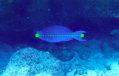
The FishSense research team was able to implement an algorithm that can take a laser dot in an image and, after thorough calibration, get the depth at that point. Then, when pointed at a fish that is perpendicular length-wise to the camera, as seen below, trigonometry can be used to get fish length. The method isn’t perfect, but it is far superior to currently used techniques.

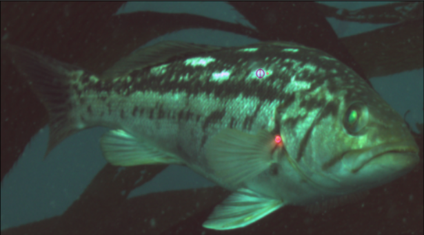
Example of how trigonometry can be used to calculate the length of a fish, given that it is perpendicular to the camera.

The problem is that it takes multiple seconds to label each laser. Each deployment returned thousands of images of fish whose lengths needed to be measured. Thus, an autonomous system to detect laser dots is necessary.

The Method:

Many different approaches were tried, to no avail. A laser dot in an image SHOULD be the brighest point, but looking for the brightest contours within an image didn’t work, but reflections of sunlight off of bubbles proved to be just as bright as the laser underwater. 2-D impulse detection, interest point detection, and edge detection all proved to be ineffective methods as well.

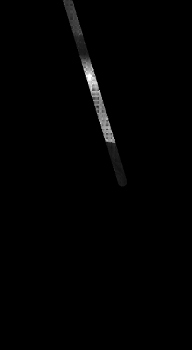
Example of a failed interest point detection, using the SIFT detector. The purple circle is the detected laser, which is clearly wrong.

Thus, I decided that this was a machine learning problem. At first, I tried a regression network. Because the laser is rigidly attached to the camera, and because the position and orientation of the laser are known, it was possible to put a “mask” over an image. The laser is guaranteed to always lie within this mask. This was just to limit the amount of information going into the network.

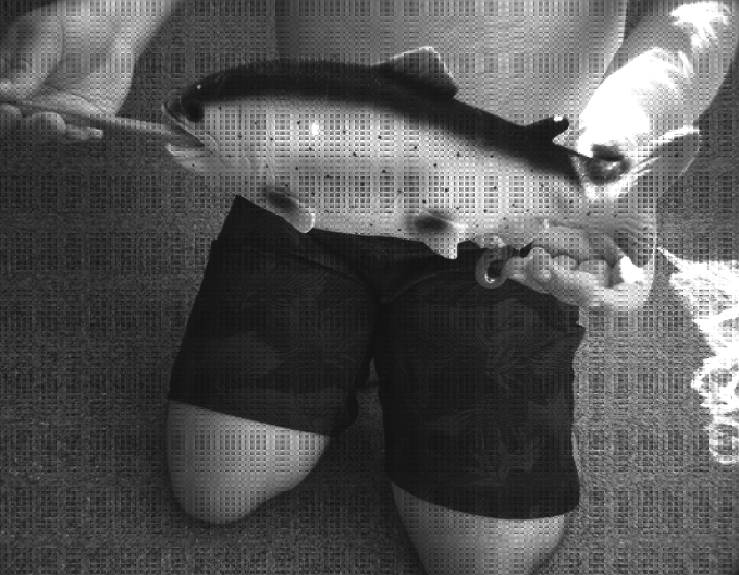
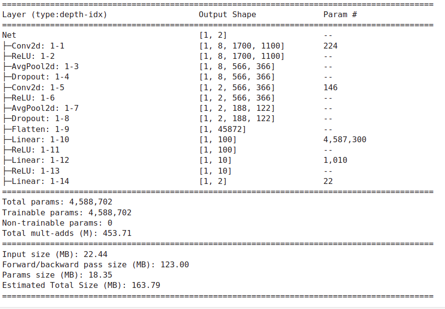
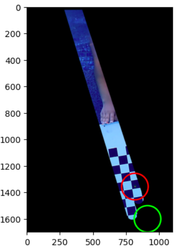
On the left is the image RAW, with the laser represented as a white dot on the fish. On the right is the same image with the mask applied on top of it. The laser dot is visible within this mask.

The regression network was fairly bulky, consisting of several convolutional and dense layers. It was trained on the few hundred images available, with the input being a masked image and the output being just 2 numbers, the x and y coordinate. After several hours of training, I realized that this approach would not work. I neglected the fact that neural networks do not behave great with regression problems, and there was just not enough data. On top of that, the model was far too large. All the predicted outputs converged to the center of the image, regardless of what image was given, as seen below.

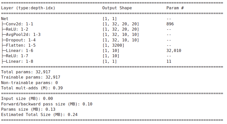
On the left is a summary of the regression model used. On the right is an example of the model failing to predict the laser. Within the red circle is the actual laser and within the green circle is the predicted laser.

My next idea was to use a binary laser or no laser classifer. Essentially, given a 20 x 20 pixel tile from the image, I wanted to create a model that could predict whether there was a laser within the image or not. In order to get training data, I took images from previous deployments and split the entire image into 20 x 20 pixel squares, so long as the square did not have a laser in it. These 20 x 20 tiles were the “no-laser” tiles. Then, I stored every single possible tile that contained the laser within it. These were the “laser” tiles. The model itself was extremely lightweight (summarized below).

On the left is a summary of the binary classifier model. On the right is an example of a laser tile.

The model itself worked super well! In deployment, however, it would be very, very costly to look at every single tile in an image. Therefore, I used a local peak finder to lower the number of options available. Local peaks within an image are the points in the image with the highest intensity. The laser is guaranteed to be a local peak, and so the idea was if I took 20 x 20 tiles around each local peak and tossed them all into the binary classifier, we’d know exactly which point was the laser. This was further augmented by only looking at local peaks within the mask.

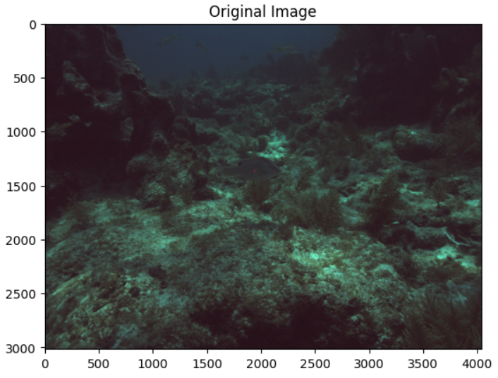
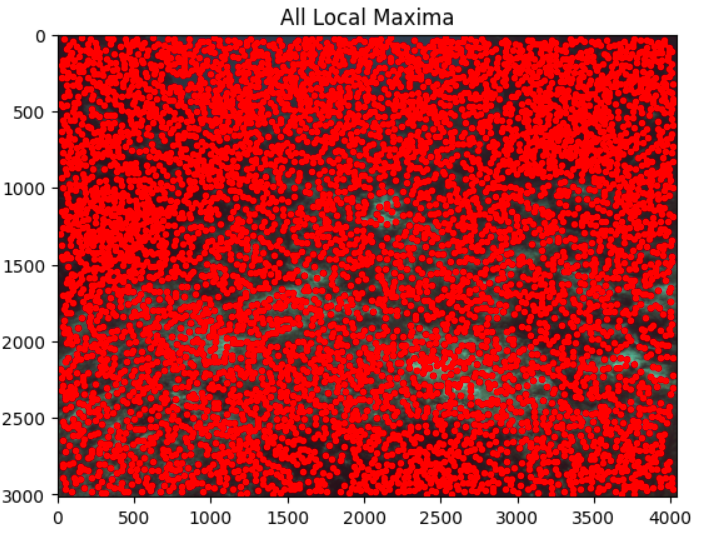
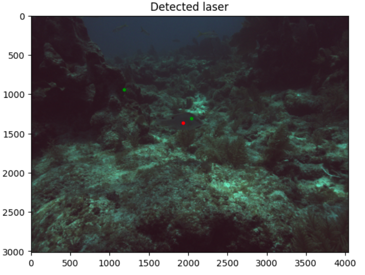
Example of the laser dot being predicted correctly. The red drawn circle is the correct prediction of the laser dot.

Ultimately, this method achieved a precision of .996 and a recall of .981, which I deemed good enough to continue on to different work.